Clustering

Clustering is the process of grouping graph elements with “similar” properties. The similarity measure is usually calculated based on topological criteria, e.g., the graph structure, or on the location of the nodes, or other characteristics, e.g., specific properties of the graph elements. Nodes that based on this similarity value are considered to be similar are grouped into the so-called Clusters. In other words, each cluster contains elements that share common properties and characteristics. The collection of all the clusters composes a clustering.

Cluster analysis has many applications fields, such as data analysis, bioinformatics, biology, big data, business, medicine. However, each of these applications may consider differently the "clustering notion," which is reflected by the fact that there exist many clustering algorithms or clustering models.

yFiles for HTML offers clustering algorithms using different kind of measures.

Using a clustering algorithm

// run a clustering algorithm, in this case biconnected component clustering.
// Note that depending on the algorithm there may be additional information
// present in the result object.
const result = new BiconnectedComponentClustering().run(graph)
for (const cluster of result.clusters) {
  const nodes = cluster.nodes
  // ...
  // do something with the nodes
  // ...
}

BiconnectedComponent

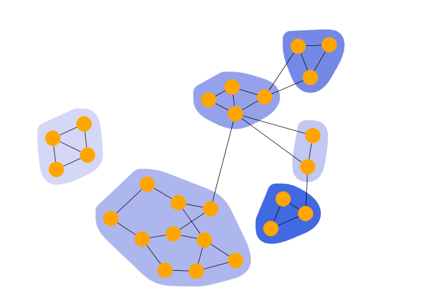
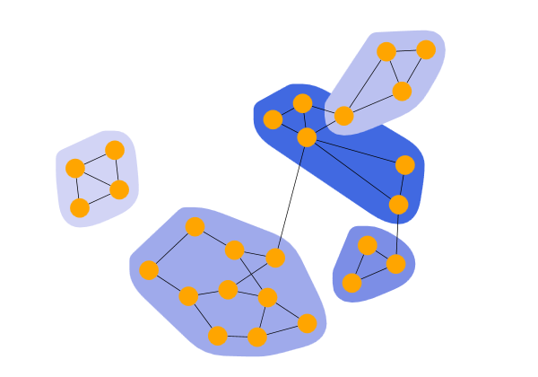
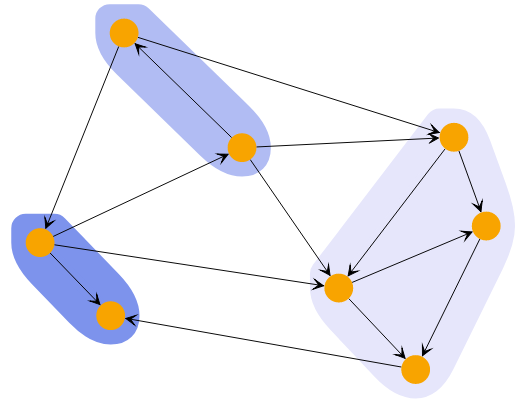
Biconnected components clustering detects clusters by analyzing the biconnected components of the graph. A biconnected component is a connected component with the property that the removal of any node keeps the component connected. Nodes of the same biconnected component form a cluster. If a node belongs to multiple biconnected components, the algorithm only assigns it to one of these clusters.

Biconnected Clusters shows the result of a BiconnectedComponentClustering that puts the nodes of each biconnected component in a cluster.

analysis clustering biconnected — Biconnected Clusters

KMeans

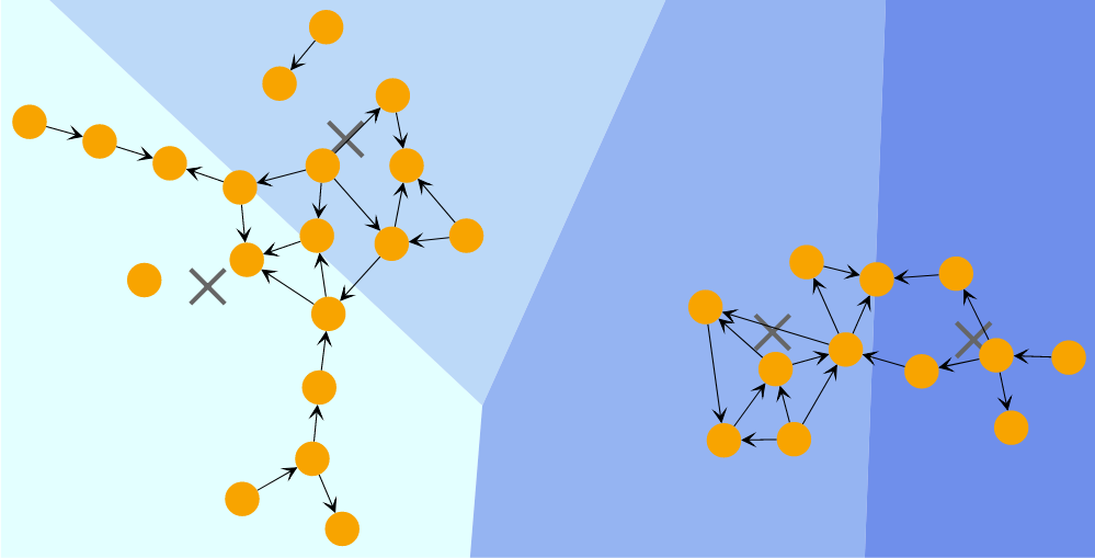
The k-Means clustering algorithm partitions the graph into k clusters based on the location of the nodes such that their distance from the cluster’s mean (centroid) is minimum. The distance is defined using various metrics as euclidean distance, euclidean-squared distance, manhattan distance, or Chebyshev distance.

K-Means Clusters shows the result of a KMeansClustering that calculates k clusters that each consist of a mean (or centroid) and all nodes closest to this mean.

analysis clustering kmeans — K-Means Clusters

EdgeBetweenness

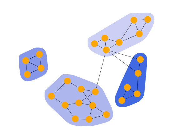
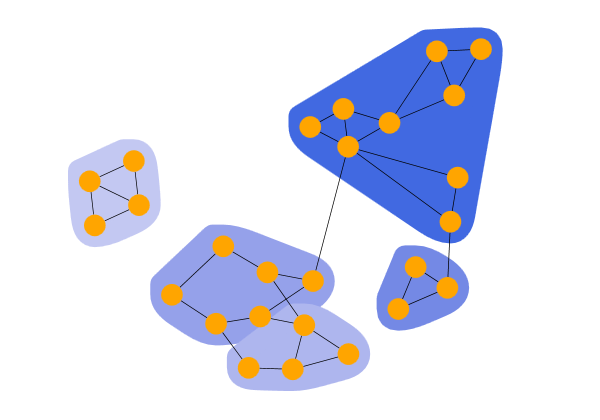
Edge Betweenness clustering detects clusters in a graph network by progressively removing the edge with the highest betweenness centrality from the graph. Betweenness centrality measures how often a node/edge lies on the shortest path between each pair of nodes in the diagram. The method stops when there are no more edges to remove or if the algorithm has reached the requested maximum number of clusters. The resulting clustering is one that achieved the best quality during the process.

Edge-Betweenness Clusters shows the result of an EdgeBetweennessClustering with a specified clusters count of 6.

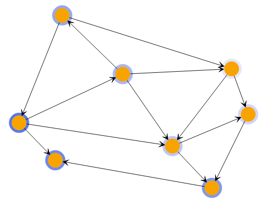
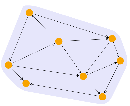
analysis clustering betweenness — Edge-Betweenness Clusters

LouvainModularity

Louvain Modularity Clustering shows the result of a LouvainModularityClustering. It starts by assigning each node to its own community/cluster. Then, it iteratively tries to construct communities by moving nodes from their current community to another until the modularity value is locally optimized. At the next step, the small communities found are merged to a single community, and the algorithm starts from the beginning until the modularity of the graph cannot be further improved.

analysis clustering louvain — Louvain Modularity Clustering

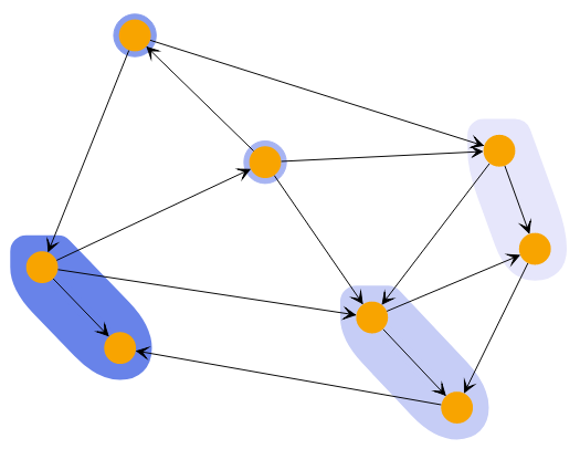
LabelPropagation

Label Propagation Clustering shows the result of a LabelPropagationClustering. The algorithm iteratively assigns a virtual label to each node. The label of a node is set to the most frequent label among its neighbors. If there are multiple candidates the algorithm randomly chooses one of them. After applying the algorithm, all nodes with the same label belong to the same community/cluster.

Hierarchical

A quite powerful way to explore the closeness of nodes in a graph is the HierarchicalClustering.

The algorithm starts by assigning each node to its own cluster and proceeds by combining the two clusters with minimal costs to a parent cluster. The cost to combine two clusters is based on a metric that is applied to each pair of nodes from the first and second cluster combined by the specified linkage. Finally, we have a hierarchy of clusters where the root cluster contains all nodes.

This hierarchy offers two ways to specify which state of the algorithm to use. You can either specify the number of clusters or the cutoff so only clusters that cost less than this value are provided.

Hierarchic Clustering with different cluster count shows clusterings of the same graph with different cluster counts.

The HierarchicalClusteringResult of the HierarchicalClustering not only provides the clusters for the initially configured clusterCount or cutoff but also the methods changeClusterCount(clusterCount: number) and changeCutoff(cutoff: number) that provide new HierarchicalClusteringResults with the changed cluster count or cutoff.

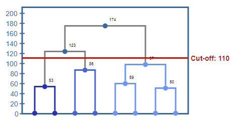
The HierarchicalClusteringResult.dendrogramRoot provides access to the root of the cluster tree that consists of DendrogramNode each representing one of the calculated clusters and providing access to the parent and children clusters.

Dendrogram of the hierarchical clustering shows the dendrogram of the cluster tree. The Cut-off value 110 results in three clusters.

analysis clustering hierarchic cutoff — Dendrogram of the hierarchical clustering

Centrality Measures Connectivity