| Advanced Layout Concepts | ||
|---|---|---|
| Prev | Chapter 5. Automatic Graph Layout | Next |
The layout algorithms that come with the yFiles library support a number of sophisticated and powerful concepts for layout generation, including:
Furthermore, many of the yFiles layout algorithms provide support for advanced inremental layout and the closely related concept of "layout from sketch." An introduction to both these concepts is presented in the section called “Incremental Layout”.
The term "grouped graph" denotes a graph structure where, conceptually, nodes can be declared "children" of a common other node, their "parent." This can be exercised recursively, i.e., parents can be declared children of other parents, resulting in a hierarchy of nodes of possibly arbitrary depth.
The visual presentation of such a hierarchy is normally done by placing the children near each other and have their parent enclosing them. The parent is called a "group node," and the children are its content, they are "grouped nodes." Declaring some nodes to be children of another node is called "grouping."
Layout support for grouped graphs primarily means proper handling of grouped nodes and their enclosing group node. The following table lists the layout algorithms that provide support for group nodes and their content:
Table 5.3. Layout support for grouped graphs
| Layout Style | Classname | Note |
|---|---|---|
| Hierarchical | IncrementalHierarchicLayouter |
IncrementalHierarchicLayouter provides direct support for grouped graphs for both incremental as well as non-incremental layout mode. See the description of IncrementalHierarchicLayouter's advanced concepts for more information. |
| Organic | SmartOrganicLayouter |
See the description of SmartOrganicLayouter's support for layout of grouped graphs for more information. |
| Orthogonal | OrthogonalGroupLayouter |
See the description of orthogonal group layout for more information. |
Table 5.4, “Routing support for grouped graphs” lists the routing algorithms that provide support for grouped graphs.
Table 5.4. Routing support for grouped graphs
| Routing Style | Classname | Note |
|---|---|---|
| Orthogonal | OrthogonalEdgeRouter |
OrthogonalEdgeRouter's support for routing with group nodes is partly handled by prepended layout stages. See the description of OrthogonalEdgeRouter for more information. Classes ChannelEdgeRouter and EdgeRouter provide inherent support for routing with group nodes. |
Further support for grouped graphs also includes minimum size constraints for group nodes. These are supported by the following layout algorithms: SmartOrganicLayouter and IncrementalHierarchicLayouter.
With an IGraph-based graph, when invoking a layout algorithm using the adapter mechanisms, all necessary setup for the layout of a grouped graph is done transparently prior to running the layout. The hierarchy of the nodes of a grouped graph, any group node insets and minimum size constraints for group nodes are converted so that a layout algorithm can access the information as supplemental data.
The two ends of an edge path are also called source port and target port, respectively. A port constraint serves to pinpoint an edge's end at its source node or target node. There are two kinds of port constraints available:
Both kinds of port constraints can easily be combined to express, for example, that an edge's source port should connect to the middle of the source node's upper border.
Table 5.5, “Layout support for port constraints” lists the layout algorithms that provide support for port constraints.
Table 5.5. Layout support for port constraints
| Layout Style | Classname | Note |
|---|---|---|
| Hierarchical | IncrementalHierarchicLayouter |
IncrementalHierarchicLayouter by default obeys weak and strong port constraints as soon as they are set. See the description of the hierarchical layout style for more information. |
| Tree | GenericTreeLayouter |
Nearly all of the predefined node placer implementations that can be used with the generic tree layout algorithm by default obey strong and weak port constraints as soon as they are set. See the description of generic tree layout for more information. |
Table 5.6, “Routing support for port constraints” lists the routing algorithms that provide support for port constraints.
Table 5.6. Routing support for port constraints
| Routing Style | Classname | Note |
|---|---|---|
| Orthogonal | OrthogonalEdgeRouter |
All classes by default obey weak and strong port constraints as soon as they are set. See the descriptions of OrthogonalEdgeRouter, ChannelEdgeRouter, BusRouter, and EdgeRouter for more information. |
Example 5.5, “Adding source port constraints to some edges (IGraph API)” demonstrates the creation of PortConstraint![]() objects, and how they are stored in an IMapper.
The mapper is then added to the mapper registry of the IGraph-based graph using
the look-up key SOURCE_PORT_CONSTRAINT_KEY
objects, and how they are stored in an IMapper.
The mapper is then added to the mapper registry of the IGraph-based graph using
the look-up key SOURCE_PORT_CONSTRAINT_KEY![]() as the mapper's tag.
During layout calculation, an algorithm first retrieves the data provider using
the look-up key, and afterwards retrieves the contained information.
as the mapper's tag.
During layout calculation, an algorithm first retrieves the data provider using
the look-up key, and afterwards retrieves the contained information.
The actual coordinates of an edge end point that has a strong port constraint associated are determined at the time a layout algorithm (or a routing algorithm) processes the edge. In other words, the strong characteristic of a strong port constraint is determined by its "normal" coordinates at the time of processing. Note that the specified coordinates of such edge end points are always interpreted relative to the respective node's center.
Example 5.5. Adding source port constraints to some edges (IGraph API)
 // 'graph' is of type com.yworks.graph.model.IGraph.

// Create a mapper.
var pcMap:IMapper = new DictionaryMapper();

// Set the coordinates for the edge's source port. (Actually, this could also
// be done anywhere prior to invoking the layout algorithm.)
graph.setPortLocation(edge3.sourcePort, -10, 20);

// Create PortConstraint objects:
// 1) Port constraint that allows an edge end to connect to any side of its
//    respective node.
var pc1:PortConstraint = PortConstraint.createWeak(PortConstraint.ANY_SIDE);
// 2) Port constraint that determines an edge end to connect *anywhere* to the
//    upper (NORTH) side of its respective node.
var pc2:PortConstraint = PortConstraint.createWeak(PortConstraint.NORTH);
// 3) Strong port constraint that determines an edge end to connect to the
//    lower (SOUTH) side of its respective node. The actual end point is at a
//    fixed coordinate.
var pc3:PortConstraint = PortConstraint.create(PortConstraint.SOUTH, true);

// Establish a mapping from edges to port constraints.
pcMap.mapValue(edge1, pc1);
pcMap.mapValue(edge4, pc2);
pcMap.mapValue(edge3, pc3);

// Add the mapper to the mapper registry of the graph.
// Use the "well-known" look-up key defined in interface PortConstraintKeys.
// Note that the above defined port constraints are set so that they apply to
// the source ends of their respective edges only.
graph.mapperRegistry.addMapper(PortConstraintKeys.SOURCE_PORT_CONSTRAINT_KEY,
    pcMap);

// Invoke the layouter.
CopiedLayoutIGraph.applyLayout(graph, new IncrementalHierarchicLayouter());
The concept of port candidates is an extension to that of classic port constraints as described above. Unlike port constraints, port candidates can be used in conjunction with both nodes and edges. When used in conjunction with nodes, port candidates provide a means to:
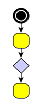
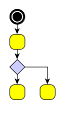
A typical example for the use of port candidates is a flow diagram as shown in Figure 5.4, “Using port candidates to control connection points”: The diamond shape, which is the visualization of a switch, should have its incoming edge connecting at the top. The first outgoing edge should connect at the bottom (left image), the second at the right, the third at the left (middle image). If there are more outgoing edges, these edges should connect at the bottom as well as more than one incoming edge should connect at the top (right image).
Figure 5.4. Using port candidates to control connection points
 |
 |
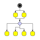 |
| Incoming edges connect at the top, the first outgoing edge at the bottom... | ... more outgoing edges occupy the right and left corners... | ... when all corners are occupied, the additional edges connect at the bottom. |
Class PortCandidate![]() enables definition
of port candidates that conceptually correspond to either weak port
constraints, i.e., effectively describe side constraints, or strong port
constraints, which encode specific anchor locations at a node.
Note that port candidates that correspond to strong port constraints directly
include the coordinates for the actual anchor locations.
enables definition
of port candidates that conceptually correspond to either weak port
constraints, i.e., effectively describe side constraints, or strong port
constraints, which encode specific anchor locations at a node.
Note that port candidates that correspond to strong port constraints directly
include the coordinates for the actual anchor locations.
PortCandidate additionally allows to associate costs with a given port candidate, which can be used to establish an order of precedence among multiple port candidates. When a given edge port is being assigned to any of the available port candidates at a node, those with low costs are favored compared to other port candidates with higher costs associated.
To define the set of side constraints and anchor locations at a node, multiple
port candidates can easily be combined using the services of class
PortCandidateSet![]() .
When a PortCandidate object is added to an instance of PortCandidateSet, the
capacity of the port candidate can optionally be configured.
The capacity of a given port candidate (sometimes also referred to as
"cardinality") specifies the allowed number of connecting edges at that side or
anchor location.
.
When a PortCandidate object is added to an instance of PortCandidateSet, the
capacity of the port candidate can optionally be configured.
The capacity of a given port candidate (sometimes also referred to as
"cardinality") specifies the allowed number of connecting edges at that side or
anchor location.
Matching port candidates means the process of distributing a node's edges to the available port candidates. All edges connecting to a node that has a set of port candidates associated with it via a PortCandidateSet object are distributed among the available port candidates with respect to:
For example, when the limit of allowed edges for a given port candidate with costs k is reached, i.e., the given port candidate is said to be "saturated," then the next least expensive port candidate among the remaining ones is chosen to connect edges to.
Example 5.6, “Defining a port candidate set” demonstrates how to create a candidate set for the diamond node shown in Figure 5.4, “Using port candidates to control connection points”: First, port candidates for the four corners of the diamond are defined. The number of connecting edges for these candidates is limited to 1. Further port candidates, which can take an unlimited number (uint.MAX_VALUE) of edges, are defined to handle any additional edges. To let the edges first connect to the corners before the additional candidates are occupied, a higher cost is associated with these latter candidates.
Example 5.6. Defining a port candidate set
// define a PortCandidateSet
var candidateSet:PortCandidateSet = new PortCandidateSet();

// the node has the size (30, 30) with the point (0, 0) at the center
// so the coordinates for the top corner are (0, -15)

// create a candidate at the top corner with direction NORTH and cost 0
var candidate:PortCandidate =
    PortCandidate.createCandidateFixedWithCost(0, -15, PortCandidate.NORTH, 0);
// add it to the set and allow only one edge to connect to it
candidateSet.addWithCapacity(candidate, 1);
// do the same for the other three corners
candidateSet.addWithCapacity(
    PortCandidate.createCandidateFixedWithCost(0, 15, PortCandidate.SOUTH, 0),
    1);
candidateSet.addWithCapacity(
    PortCandidate.createCandidateFixedWithCost(15, 0, PortCandidate.EAST, 0),
    1);
candidateSet.addWithCapacity(
    PortCandidate.createCandidateFixedWithCost(-15, 0, PortCandidate.WEST, 0),
    1);

// to allow more edges to connect at the top and bottom
// create extra candidates and allow uint.MAX_VALUE edges to connect

// to avoid that these candidates are occupied before the others
// associate a cost of 1 with them
candidateSet.addWithCapacity(
    PortCandidate.createCandidateFixedWithCost(0, -15, PortCandidate.NORTH, 1),
    uint.MAX_VALUE);
candidateSet.addWithCapacity(
    PortCandidate.createCandidateFixedWithCost(0, 15, PortCandidate.SOUTH, 1),
    uint.MAX_VALUE);
To influence the matching process, a subset of the PortCandidate objects used
for a node can additionally be associated with the respective ports of its
connecting edges.
The subset then defines a restricted set of desired port candidates an edge
prefers to connect to.
The PortCandidate objects can be combined using Collection![]() objects which are stored by means of data providers.
The data providers are registered with the graph using the look-up keys
SOURCE_PCLIST_DPKEY
objects which are stored by means of data providers.
The data providers are registered with the graph using the look-up keys
SOURCE_PCLIST_DPKEY![]() and
TARGET_PCLIST_DPKEY
and
TARGET_PCLIST_DPKEY![]() .
.
Table 5.7, “Layout support for port candidates” lists the layout algorithms that provide support for port candidates.
Table 5.7. Layout support for port candidates
| Layout Style | Classname | Note |
|---|---|---|
| Hierarchical | IncrementalHierarchicLayouter |
IncrementalHierarchicalLayouter supports port candidates as soon as they are set. See the description of incremental hierarchical layout for more information. |
The PortCandidateSet objects for the node set of a graph can be registered by adding
an IMapper to the mapper registry of an IGraph-based graph using the NODE_DP_KEY![]() data provider look-up key as the mapper's tag.
data provider look-up key as the mapper's tag.
Example 5.7. Registering candidates (IGraph API)
// 'candidateSet' is of type com.yworks.yfiles.layout.PortCandidateSet
// 'node' is of type com.yworks.graph.model.INode and is the node which should
// be associated with the candidate set
// 'graph' is of type com.yworks.graph.model.IGraph.

// Create a mapper to associate the candidates with the node.
var pcMap:IMapper = new DictionaryMapper();
// Associate the candidate set with the node.
pcMap.mapValue(node, candidateSet);

// Add the mapper to the mapper registry of the graph.
graph.mapperRegistry.addMapper(PortCandidateSet.NODE_DP_KEY, pcMap);
The same scheme of combining PortCandidate objects using Collection objects as used for the matching functionality also enables creating enhanced port constraint definitions for edges. The layouters which support this feature are listed in Table 5.8, “Layout support for enhanced port candidates”.
Table 5.8. Layout support for enhanced port candidates
| Layout Style | Classname | Note |
|---|---|---|
| Hierarchical | IncrementalHierarchicLayouter |
IncrementalHierarchicalLayouter supports port candidates as soon as they are set. See the description of incremental hierarchical layout for more information. |
In particular, this scheme is supported by yFiles routing algorithms, and it allows to conveniently specify side constraints comprising two or three sides, for example. Table 5.9, “Routing support for port candidates” lists the routing algorithms that provide support for port candidates modeling enhanced port constraints.
Table 5.9. Routing support for port candidates
| Routing Style | Classname | Note |
|---|---|---|
| Orthogonal | OrthogonalEdgeRouter |
All classes by default support port candidates as soon as they are set. See the descriptions of OrthogonalEdgeRouter, ChannelEdgeRouter, BusRouter, and EdgeRouter for more information. |
Example 5.8, “Creating enhanced port constraints using port candidates (IGraph API)” shows how port candidates can be used to model enhanced port constraints that allow the source port of edges to connect to two sides of the start nodes.
Example 5.8. Creating enhanced port constraints using port candidates (IGraph API)
public class MyConstIMapper implements IMapper {

  private var _value:Object;

  function MyConstIMapper(value:Object) {
    this._value = value;
  }

  public function lookupValue(key:Object):Object {
    return (key is IEdge ? _value : null);
  }

  public function mapValue(key:Object, value:Object):void {}

  public function unMapValue(key:Object):void {}
}

// 'graph' is of type com.yworks.graph.model.IGraph.

// Define a collection of port candidates for the source ports of all edges.
var pcc:Collection = new ArrayList();
// Create port candidates that conceptually correspond to classic side
// constraints (weak constraints) and add them to the collection.
// East side.
pcc.addItem(PortCandidate.createCandidate(PortCandidate.EAST));
// South side.
pcc.addItem(PortCandidate.createCandidate(PortCandidate.SOUTH));

// Create a data provider (adapter) that returns the collection of port
// candidates for each edge.
// Use the "well-known" look-up key defined in class PortCandidate.
graph.mapperRegistry.addMapper(PortCandidate.SOURCE_PCLIST_DPKEY,
                               new MyConstIMapper(pcc));

// Invoke an edge routing algorithm.
CopiedLayoutIGraph.applyLayout(graph, new OrthogonalEdgeRouter());
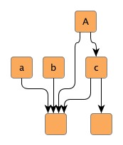
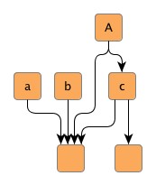
Edge grouping means bundling of a set of edges to be treated in a common manner regarding some aspects of edge path generation. Specifically, if edges at a common source node, for example, are declared an edge group at their source ends, then their source ports will be anchored at the same location.
Additionally, all grouped edges will also be routed in bus-style, i.e., their paths will share a common edge segment. If edges at different source (target) nodes are declared an edge group at their source (target) ends, then they will be routed in bus-style only.
Figure 5.5. Edge groups
 |
 |
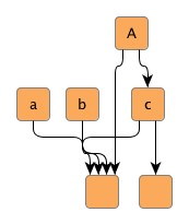 |
| Hierarchical layout without any edge groups, ... | ... with an edge group at the source ends of outgoing edges at node A. The source ports are anchored at the same location. Also, the edges are routed in bus-style, i.e., their paths share a common edge segment. | ... with an edge group at the source ends of outgoing edges at node a, b, and c. The edges are routed in bus-style, i.e., their paths share a common edge segment. |
Declaring an edge group at either source or target ends of a set of edges is done
by associating a common object with the edges via a data provider.
Depending on which end the edge group is declared for, an IMapper is added to the
mapper registry of the IGraph-based graph using either the
SOURCE_GROUPID_KEY![]() or
TARGET_GROUPID_KEY
or
TARGET_GROUPID_KEY![]() look-up key as the mapper's tag.
look-up key as the mapper's tag.
Edge grouping is also referred to as port grouping sometimes. If edges from an edge group have associated inconsistent, or even contradicting port constraints, then the location of the common port is not guaranteed to obey any of them.
Table 5.10, “Layout support for edge groups” lists the layout algorithms that provide support for edge groups.
Table 5.10. Layout support for edge groups
| Layout Style | Classname | Note |
|---|---|---|
| Hierarchical | IncrementalHierarchicLayouter |
IncrementalHierarchicLayouter by default generates edge/port groups as soon as they are declared. See the description of the hierarchical layout style for more information. |
| Orthogonal | DirectedOrthogonalLayouter |
The directed orthogonal layout algorithm by default generates edge/port groups as soon as they are declared. See the description of directed orthogonal layout for more information. |
| Series-parallel | SeriesParallelLayouter |
The series-parallel layout algorithm by default generates edge/port groups as soon as they are declared. See the description of series-parallel layout for more information. |
Table 5.11, “Routing support for edge groups” lists the routing algorithms that provide support for edge groups.
Table 5.11. Routing support for edge groups
| Routing Style | Classname | Note |
|---|---|---|
| Orthogonal | OrthogonalEdgeRouter |
OrthogonalEdgeRouter's support for edge/port groups is partly handled by prepended layout stages. See the description of OrthogonalEdgeRouter for more information. Class EdgeRouter provides inherent support for edge/port groups. |
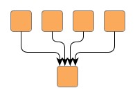
Example 5.9, “Creating an edge group at a common target node (IGraph API)” demonstrates how edge groups are
declared, and how an IMapper is added to the mapper registry of the IGraph-based
graph using the look-up key TARGET_GROUPID_KEY![]() as the mapper's tag.
During layout calculation, an algorithm first retrieves the data provider using
the look-up key, and afterwards retrieves the contained information.
as the mapper's tag.
During layout calculation, an algorithm first retrieves the data provider using
the look-up key, and afterwards retrieves the contained information.
Figure 5.6. Edge group at a common target node
 |
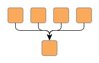 |
| Hierarchical layout without any edge groups... | ... and with an edge group at the target ends of the edges. All target ports are anchored at the same location at the common node. Also, the edges are routed in bus-style, i.e., their paths share a common edge segment. |
Example 5.9. Creating an edge group at a common target node (IGraph API)
// 'graph' is of type com.yworks.graph.model.IGraph.
// 'specificNode' is of type com.yworks.graph.model.INode.

// Create a mapper.
var egMap:IMapper = new DictionaryMapper();

// Declare an edge group for the target end of all incoming edges at a specific
// node.
var targetEdgeGroupID:String = "All my grouped edges.";
for (var it:Iterator = graph.edgesAtPortOwner(specificNode).iterator();
     it.hasNext(); ) {
  var e:IEdge = IEdge(it.next());
  egMap.mapValue(e, targetEdgeGroupID);
}

// Add the mapper to the mapper registry of the graph.
// Use the "well-known" look-up key defined in class PortConstraintKeys as tag.
graph.mapperRegistry.addMapper(PortConstraintKeys.TARGET_GROUPID_KEY, egMap);

// Invoke the layouter.
CopiedLayoutIGraph.applyLayout(graph, new IncrementalHierarchicLayouter());
For the calculation of partitioned layouts, i.e., in particular the special case of swimlane layouts, the so-called partition grid provides the necessary support.
Class PartitionGrid![]() encapsulates a simple grid-like structure consisting of rows and columns.
In addition to the structure itself, the partition grid also holds geometric information
related to both rows and columns, like, e.g. minimum heights/widths or insets.
encapsulates a simple grid-like structure consisting of rows and columns.
In addition to the structure itself, the partition grid also holds geometric information
related to both rows and columns, like, e.g. minimum heights/widths or insets.
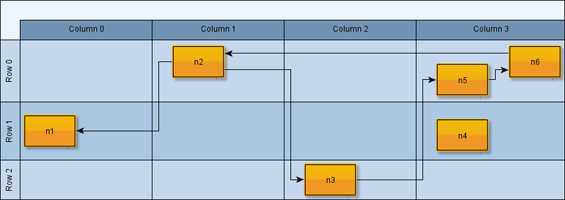
Figure 5.7, “Partition grid” shows a partitioned layout. Note the two-dimensional partition which results from the rows and columns.
The geometric information specific to a row or column is available through its descriptor
object, which is an instance of RowDescriptor![]() or ColumnDescriptor
or ColumnDescriptor![]() ,
respectively.
,
respectively.
Table 5.12, “Layout support for swimlane/partitioned layout” lists the layout algorithms that provide support for swimlane/partitioned layout.
Table 5.12. Layout support for swimlane/partitioned layout
| Layout Style | Classname | Note |
|---|---|---|
| Hierarchical | IncrementalHierarchicLayouter |
IncrementalHierarchicLayouter provides direct support for swimlane/partitioned layout. See the description of IncrementalHierarchicLayouter's support for Swimlane Layout for more information. |
| Organic | SmartOrganicLayouter |
SmartOrganicLayouter provides direct support for swimlane/partitioned layout. See the description of Partitioned Layout for more information. |
The setup for swimlane/partitioned layout calculation of a graph with table structures
is a matter of using the convenience methods of class TableLayoutConfigurator![]() as shown in Example 5.10, “Swimlane/partitioned layout preparation”.
as shown in Example 5.10, “Swimlane/partitioned layout preparation”.
Example 5.10. Swimlane/partitioned layout preparation
// 'graph' is of type com.yworks.graph.model.IGraph.
// 'graphCanvas' is of type com.yworks.ui.GraphCanvasComponent.

// Configure IncrementalHierarchicLayouter.
var ihl:IncrementalHierarchicLayouter = new IncrementalHierarchicLayouter();
ihl.componentLayouterEnabled = false;
ihl.layoutOrientation = LayoutOrientation.LEFT_TO_RIGHT;
ihl.orthogonalRouting = true;
ihl.recursiveGroupLayering = false;
SimplexNodePlacer(ihl.nodePlacer).baryCenterMode = true;

try {
  var tlc:TableLayoutConfigurator = new TableLayoutConfigurator();
  tlc.compactionEnabled = false;
  tlc.horizontalLayout = true;
  tlc.fromSketch = true;

  // Prepare all relevant information for a layout algorithm.
  tlc.prepareAll(graph);
  // Start layout calculation.
  CopiedLayoutIGraph.applyLayout(graph, ihl);
  tlc.restoreAll(graph);
}
catch (exception:Error) {
  trace(exception);
}
Setup code can be reduced to a minimum by using convenience class LayoutExecutor, which also takes care of all necessary configuration steps related to swimlane/partitioned layout.
Example 5.11, “Swimlane/partitioned layout preparation (IGraph API)” demonstrates how to set up a swimlane/partitioned layout without the convenience functionality from class TableLayoutConfigurator.
The services of the PartitionGrid![]() class
can be used to
class
can be used to
Partitioned layout calculation needs a PartitionGrid object registered via a data
provider with the graph using look-up key PARTITION_GRID_DPKEY![]() and the mapping of the nodes to partition cells registered via data provider with
the graph using look-up key PARTITION_CELL_DPKEY
and the mapping of the nodes to partition cells registered via data provider with
the graph using look-up key PARTITION_CELL_DPKEY![]() .
During layout calculation, an algorithm first retrieves the data providers using
the look-up keys, and afterwards retrieves the contained information.
.
During layout calculation, an algorithm first retrieves the data providers using
the look-up keys, and afterwards retrieves the contained information.
Basically, the partition grid needs to be created, and the data providers that hold the necessary information about the partition grid and the mapping of nodes to cells have to be filled manually, and be registered with the graph using the data provider look-up keys defined in class PartitionGrid.
Example 5.11. Swimlane/partitioned layout preparation (IGraph API)
// 'graph' is of type com.yworks.graph.model.IGraph.
// 'n1' to 'n6' are of type com.yworks.graph.model.INode.

// Create a grid having three rows and four columns.
var grid:PartitionGrid = PartitionGrid.newPartitionGrid2(3, 4);

// Create an IMapper to store the mapping of nodes to swimlanes, resp. partition
// grid cells.
var cellMap:IMapper = new DictionaryMapper();

// Assign the nodes to the cells.
cellMap.mapValue(n1, grid.createCellId2(1, 0));
cellMap.mapValue(n2, grid.createCellId2(0, 1));
cellMap.mapValue(n3, grid.createCellId2(2, 2));
cellMap.mapValue(n4, grid.createCellId2(1, 3));
cellMap.mapValue(n5, grid.createCellId2(0, 3));
cellMap.mapValue(n6, grid.createCellId2(0, 3));

// Add the PartitionGrid object and the mapper to the mapper registry of the
// graph.
// Use the "well-known" look-up keys defined in class PartitionGrid as tags.
var mapperRegistry:IMapperRegistry = graph.mapperRegistry;
mapperRegistry.addMapper(PartitionGrid.PARTITION_GRID_DPKEY,
                         new MyConstantMapper(grid));
graph.mapperRegistry.addMapper(PartitionGrid.PARTITION_CELL_DPKEY, cellMap);

// Create the layout algorithm...
var ihl:IncrementalHierarchicLayouter = new IncrementalHierarchicLayouter();
ihl.layoutOrientation = LayoutOrientation.LEFT_TO_RIGHT;
// ... and start layout calculation.
CopiedLayoutIGraph.applyLayout(graph, ihl);
Note that Example 5.11, “Swimlane/partitioned layout preparation (IGraph API)” shows the basic setup of the partition grid seen in Figure 5.7, “Partition grid”. Observe how the layout algorithm respects the specified organization of the nodes within the partition cells.
To create IDs for the cells of a partition (single cells and ranges of cells), class PartitionGrid provides the methods below. The IDs can be used to assign the nodes of a diagram to partition cells. Nodes that do not have an ID associated, can be placed in any partition cell by a layout algorithm.
createCellId2(rowIndex:int, colIndex:int):PartitionCellId |
|
| Description | Creates partition IDs for single cells. |
createCellSpanId2(fromRowIndex:int, fromColIndex:int, toRowIndex:int, toColIndex:int):PartitionCellId |
|
| Description | Creates partition IDs that represent a (two-dimensional) range of cells stretching the specified rows and columns. |
In the set of all specified cells of a partition (single cells and ranges of cells), no two ranges of cells are allowed to overlap with each other, or overlap with a single cell, i.e., the set needs to be disjoint. In particular, this also means that no partition cell can have more than one partition ID associated with it.
Class PartitionGrid enables further optimization of the layout outcome when there are no cell spans specified in a partition grid. The following properties can be used to control whether the order of rows and columns in a swimlane/partitioned layout shall be automatically determined.
optimizeRowOrder:Boolean |
|
| Description | Optimize the order of rows to minimize the diagram's overall edge lengths. |
optimizeColumnOrder:Boolean |
|
| Description | Optimize the order of columns to minimize the diagram's overall edge lengths. |
A node halo basically specifies additional paddings around a node. A layout algorithm that supports node halos, keeps this area clear of graph elements, except the labels of this specific node and the adjacent segments of its edges.
Class NodeHalo![]() can be used to denote a node's
additional size requirements.
The NodeHalo objects for the node set of a graph can be registered by adding an
IMapper to the mapper registry of an IGraph-based graph using the NODE_HALO_DPKEY
can be used to denote a node's
additional size requirements.
The NodeHalo objects for the node set of a graph can be registered by adding an
IMapper to the mapper registry of an IGraph-based graph using the NODE_HALO_DPKEY![]() data provider look-up key as the mapper's tag.
data provider look-up key as the mapper's tag.
The following layout algorithms provide support for node halos:
Table 5.13. Layout support for node halos
| Layout Style | Classname | Note |
|---|---|---|
| Hierarchical | IncrementalHierarchicLayouter |
IncrementalHierarchicLayouter by default obeys node halos as soon as they are declared. See the description of the hierarchical layout style for more information. |
| Orthogonal | OrthogonalLayouter |
All classes by default support node halos as soon as they are declared.
See the descriptions of
OrthogonalLayouter,
OrthogonalGroupLayouter, and
DirectedOrthogonalLayouter
for more information.
Note that CompactOrthogonalLayouter |
| Tree | TreeLayouter |
All classes by default support node halos as soon as they are declared. See the descriptions of TreeLayouter, BalloonLayouter, and GenericTreeLayouter for more information. |
| Circular | CircularLayouter |
CircularLayouter by default obeys node halos as soon as they are declared. See the description of the circular layout algorithm for more information. |
| Organic | SmartOrganicLayouter |
SmartOrganicLayouter by default obeys node halos as soon as they are declared. See the description of the organic layout algorithm for more information. |
| Radial | RadialLayouter |
RadialLayouter by default obeys node halos as soon as they are declared. See the description of the radial layout algorithm for more information. |
The following routing algorithms provide support for node halos:
Table 5.14. Routing support for node halos
| Routing Style | Classname | Note |
|---|---|---|
| Orthogonal | EdgeRouter |
Class EdgeRouter provides inherent support for node halos. |
|
Copyright ©2010-2015, yWorks GmbH. All rights reserved. |